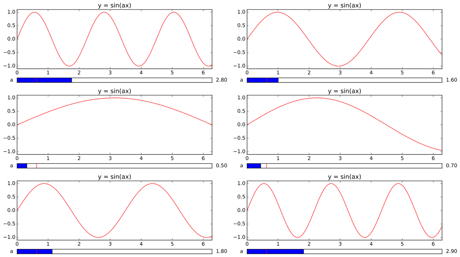
Matplotlib slider widget

Using matplotlib we can create not only static graphs, but also graphs that can be modified interactively. Tools for this are contained in the widgets submodule. Here we will use the Slider widget to create a plot of a function with a scroll bar that can be used to modify the plot:

This animation shows the graph of the function \(y = sin(ax)\) for various values of a parameter \(a\). The value of the parameter is modified by scrolling the slider. Here is the code that creates this interactive plot:

from matplotlib.widgets import Slider  # import the Slider widget

import numpy as np
import matplotlib.pyplot as plt
from math import pi

a_min = 0    # the minimial value of the paramater a
a_max = 10   # the maximal value of the paramater a
a_init = 1   # the value of the parameter a to be used initially, when the graph is created

x = np.linspace(0, 2*pi, 500)

fig = plt.figure(figsize=(8,3))

# first we create the general layount of the figure
# with two axes objects: one for the plot of the function
# and the other for the slider
sin_ax = plt.axes([0.1, 0.2, 0.8, 0.65])
slider_ax = plt.axes([0.1, 0.05, 0.8, 0.05])


# in plot_ax we plot the function with the initial value of the parameter a
plt.axes(sin_ax) # select sin_ax
plt.title('y = sin(ax)')
sin_plot, = plt.plot(x, np.sin(a_init*x), 'r')
plt.xlim(0, 2*pi)
plt.ylim(-1.1, 1.1)

# here we create the slider
a_slider = Slider(slider_ax,      # the axes object containing the slider
                  'a',            # the name of the slider parameter
                  a_min,          # minimal value of the parameter
                  a_max,          # maximal value of the parameter
                  valinit=a_init  # initial value of the parameter
                 )

# Next we define a function that will be executed each time the value
# indicated by the slider changes. The variable of this function will
# be assigned the value of the slider.
def update(a):
    sin_plot.set_ydata(np.sin(a*x)) # set new y-coordinates of the plotted points
    fig.canvas.draw_idle()          # redraw the plot

# the final step is to specify that the slider needs to
# execute the above function when its value changes
a_slider.on_changed(update)

plt.show()

Note. Code similar to the one above will work fine for plots with one slider, but if we want two have two (or more) sliders controlling various parameters of the plot, it will require a modification. The problem is that in such situation we may need to use in the update() function values coming from different sliders, but this function must have exactly one argument. This can be fixed as follows. A slider slider_name has an associated variable slider_name.val that stores the current value of the slider. This variable can be used in the update() function to get the value of the slider and modify the plot. For example, in the code above the update() function can be changed as follows:

def update(a):
    sin_plot.set_ydata(np.sin(a_slider.val*x)) # set new y-coordinates of the plotted points
    fig.canvas.draw_idle()          # redraw the plot

Here a_slider is the name of the slider, so a_slider.val gives the the current value of this slider. If the plot had another slider b_slider then we could use b_slider.val to the get the value of that slider and use it in the update() function.

Exercise 1. Lissajous curves are curves given by the parametric equations

\[x = \sin(at)\]

\[y = \cos(bt)\]

Create an interactive plot of Lissaous curves with two sliders: one controlling the paramater \(a\) and the other controlling \(b\).

The widgets submodule of matplotlib contains many other tools, beside slider, that can be used to add interactive features to plots (buttons, radio buttons, check boxes etc.). See matplotlib documentation for details.